تم الحل ✓
categoryالهندسة الميكانيكية
schoolبكالوريوس
event_available2026-07-14
السؤال
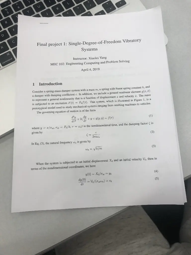
Transcribed Image Text:
D
R
"
%
5
A
6
Y
U
K
L
command
Final project 1: Single-Degree-of-Freedom Vibratory
Systems
Instructor: Xiaolei Yang
MEC 102: Engineering Computing and Problem Solving
April 4, 2019
1 Introduction
Consider a spring-mass-damper system with a mass m, a spring with linear spring constant k, and
a damper with damping coefficient c. In addition, we include a general nonlinear element g(x, z)
to represent a general nonlinearity that is a function of displacement and velocity . The mass
is subjected to an excitation F(t) = Fof(t). This system, which is illustrated in Figure 1, is a
prototypical model used to study mechanical systems ranging from washing machines to vehicles.
The governing equation of motion is of the form
d'y
+24 +y+9(y.y) f(T)
مولی
dy
dr
(1)
where y=x/st, st = Fo/k, wat is the nondimensional time, and the damping factor ( is
given by
!
2mwa
In Eq. (3), the natural frequency w,, is given by
√k/m
(2)
(3)
When the system is subjected to an initial displacement X, and an initial velocity Vo, then in
terms of the nondimensional coordinates, we have
y(0) = Xo/ost = yo
dy(0)
==
Vo/(0) =
=20
dT
(4)
(5)
x(1)
F(1) = Fof(t)
ни
m
g(x,x)
2
Figure 1: Spring-mass-damper system with a general nonlinear element g(x, z).
Example: System with nonlinear spring and forced oscilla-
tions
For this system, there is a nonlinear cubic spring with spring constant, thus,
where
9(3.9)=aoy",
(6)
Q=
(7)
k
The initial conditions are zero. The harmonic forcing at frequency w is given by
F(T) Fo cos(wt) = Fa cos(r)
(8)
where = w/w is the nondimensional excitation frequency ratio. Substitute Eqs. (6) and (8) into
Eq. (1), the governing equation is obtained as follows:
d²y
dy
dr²
+26+y+aoy³ = cos(fr)
Introducing the following variables
Y₁ = y
dy
32.
(9)
(10)
-velocity
(11)
Eq. (9) becomes
dy
(12)
= y2
dT
dy2
-2y-1-a0 + cos(T),
(13)
dr
and
91 (0) = 0
92 (0) = 0,
(14)
(15)
9
10
11
12
13
ONDERST
14
15
16
17
18
19
At a given excitation frequency, we shall determine the steady-state response of the system
given by Eq. (9)-that is, after the transients have died out-and examine the spectral content of this
steady-state response employing fft for the following cases: (1) a = 0 (linear system) and (2)
6,250 (nonlinear system).
Equation (9) is numerically integrated using ode45. In addition, we assume that (=0.2 and
?= 3.0. The excitation frequency 2 has been chosen to be three times the natural frequency of
the system. We shall examine the time histories for 0≤30 and take 12,000 samples in this
region. This is equivalent to the data being acquired every T, = 30/12,000 = 0.0025. Therefore,
the (dimensionless) sampling frequency is 2/7T,800. This is far in excess of what is necessary
to sample the response based on the excitation frequency = 3.0. The consequence of this over-
sampling is that we have to truncate the spectrum plot; thus, we shall display only the first forty
3,200 and the number of samples used by fit is N = 2138, 192.
values. Also, we let Natart
The script is as follows:
1 function Example01
0.2; alphao = [0, 62501;
3; M =12000;
linspace (0, 30, M);
N = 2 13; Nstart = 3200; Fs = M/30;
2
zeta =
3
Omega
E
4
tspan =
5
6
7
8
f = (Fs (0:N-1)/N) *2.0*pi;
for m = 1:2
[t, y] = ode 45 (@ForcedNLOscillator, tspan, [0
0]');
figure (m);
plot (t, y(:,1), 'k-');
axis ([0, 25, -0.2, 0.46]);
xlabel(’\tau);
ylabel(’y(\tau));
axes ('position', [0.55, 0.63, 0.25, 0.25])
Amp = abs (fft (y (Nstart: Nstart+N, 1), N))/N;
plot (f (1:40), 2*Amp (1:40), 'k-');
v = axis; v (2) = f (40); v(4) =
max (2*Amp (1:40)); axis (v)
xlabel('\Omega');
ylabel('Amplitude');
21
end
function xdot =
ForcedNLOscillator (t, x)
22
23
22
24 end
end
xdot = [x (2); -2*zeta*x (2) -x (1) -
alphao (m) *x (1) ^3+cos (Omega*t)];
Execution of the program results in Figure 2, where it is seen that the responses of both the
linear and nonlinear systems reach steady state when r≥ 8. This time corresponds to an index
Natart =3,200. Although both of the steady-state responses have a period equal to the period of the
harmonic forcing function, they have different characteristics that can be more clearly distinguished
in the frequency domain. The corresponding spectral response appears in the upper right-hand cor-
ner of each figure where it is seen that the amplitude spectrum of the displacement response in the
nonlinear case shows spectral peaks at the forcing frequency 2 and at integer multiples of it. The
additional peaks are due to the cubic nonlinearity of the spring. In the linear case, there is only
one spectral peak, which corresponds to the excitation frequency. This example illustrates that the
response of a nonlinear system can have spectral components different from the excitation (input)
frequency.
3 Problem for final project 1
An overhead crane's trolley is carrying, via a cable, a load of mass m as shown in Figure 3. When
the trolley is moved with an acceleration b(t), the governing equation of motion of the crane load
is
d20
L-
dt2
+g sin(0)-b(t) cos(0)
(16)
where 9 = 9.8m/s2 is the gravity constant. If the cable length is L = 2 m, then graph the swing
motion (t) for the following accelerations of the trolley over the time interval 0 <t<10 s:
1. b(t) = 10u(t) m/s², 0(0) = 0.4 rad, and de(0)/dt = 0.1 rad/s, where u(t) is the unit step
function.
2. b(t)=0.2u(t) m/s², 0(0) = 0.4 rad, and de(0)/dt = 0.1 rad/s, where u(t) is the unit step
function.
1
You need to submit: 1) the MATLAB code, and 2) the images.
0.4-
0.1
0.3
0.2-
0.1
-0.1-
0.05
5
10
9
-0.2
10
15
20
25
0.4-
(a)
0.04
0.3-
0.02
0.2
0.1-
-0.1-
5
10
..
-0.25
10
15
20
25
T
(b)
Figure 2: (a) Linear system subjected to a harmonic forcing at 2 = 3.(b) Nonlinear system sub-
jected to a harmonic forcing at = 3 and 0 = 6,250.
Trolley
•
b(t)
m
L
k
IC = XCQ)=xo J
9C44)-8048
-FCT) =Focos (7)
Crane boom
Figure 3: Trolley on an overhead crane carrying a swinging load m.
check_circle الجواب — حل مفصل خطوة بخطوة
hourglass_top
🔒
الحل الكامل متاح للمشتركين
اشترك في أرشيف الأسئلة لعرض هذا الحل وآلاف الحلول المفصلة خطوة بخطوة من معلمين معتمدين.