تم الحل ✓
categoryهندسة ميكانيكية
schoolبكالوريوس
event_available2026-07-14
السؤال
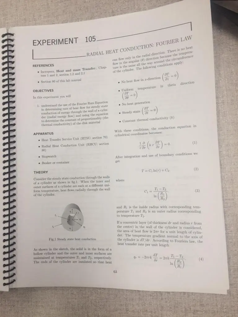
Transcribed Image Text:
EXPERIMENT 105.
REFERENCES
RADIAL HEAT CONDUCTION: FOURIER LAW
Incropers, Heat and mass Transfer.. Chap-
ters 1 and 2, section 1.2 and 2.1
Section 80 of this lab manual
OBJECTIVES
In this experiment you will
1. understand the use of the Fourier Rate Equation a
in determining rate of heat flow for steady state
conduction of energy through the wall of a cylin-
der (radial energy flow) and using the equation
to determine the constant of proportionality (the
thermal conductivity) of the disk material
APPARATUS
Heat Transfer Service Unit (HTSU: section 70)
Radial Heat Conduction Unit (RHCU: section
80)
Stopwatch
Beaker or container
can flow only in the radial direction. There is no heat
flow in the angular (0) direction because the tempera-
ture is the same all the way around the circumference
of the cylinder. The following conditions apply:
No heat flow in z-direction
ยะ
Uniform temperature in theta
OT
=0
No heat generation
• Steady state
(-)
Constant thermal conductivity (k)
direction
With these conditions, the conduction equation in
cylindrical coordinates becomes:
10
()-
=0.
T
(1)
After integration and use of boundary conditions we
get
THEORY
Consider the steady state conduction through the walls
of a cylinder as shown in fig.1. When the inner and
outer surfaces of a cylinder are each at a different uni-
form temperature, heat flows radially through the wall
of the cylinder.
T=C₁ In(r) +C2.
where
T-T
C₁ =
R₁
In
R₂
(3)
Fig.1 Steady state heat conduction
As shown in the sketch, the solid is in the form of a
hollow cylinder and the outer and inner surfaces are
maintained at temperatures T and Ty, respectively.
The ends of the cylinder are insulated so that heat
and R₁ is the inside radius with corresponding tem-
perature T and R₁ is an outer radius corresponding
to temperature T
If a concentric layer (of thickness dr and radius r from
the centre) in the wall of the cylinder is considered,
the area of heat flow is 2rr for a unit length of cylin-
der. The temperature gradient normal to the axis of
the cylinder is dT/dr. According to Fouriers law, the
heat transfer rate per unit length
9r=-2ark =2k
8T
бр
T-T₂
R₂
(4)
In
R₁
63
APPA
E
Li
70
Ste
Be
THEORY
Consider t
as shown i
and Cand
ness L, w
convect he
side may b
environmen
infy the bes
is a linear i
following so
Considering a cylinder of length I. and rearranging the
the last equation we get:
T-T
Q-2rkl
Ra
In
R
In
2rkL (T-T)
(6)
The heat flow path in the RHCU consists of a cylinder
3.2 mm long (thickness of disk Z) with inside radius
R-7 mm (where thermocouple T is located) and
outer radius Re-50 mm (where thermocouple To is
located). The objective of this exercise is to determine
the conductivity of the disk material from measure-
ments of temperature difference and heat flow through
the cylindrical disk.
PROCEDURE
Fig. 1 Radial beat conduction
1. Connect the thermocouples to the appropriate
sockets on the front of the service unit.
2. Start the computer. Start the heat transfer.
service unit (HTSU) using the power switch
MAINS. Set the selector switch to "Automatic",
then start the ArmSoft software and select "Ex-
ercise B.
3. The Mimic Diagram is the most commonly used
display of the software, it gives a pictorial rep
resentation of the equipment, with continuously
updated display boxes for all the various sensor
readings, calculated variables etc. To view the
Mimic Diagram, click Diagram from the View
drop down menu.
4. In order to establish communication between the
software and HTSU, click on the "Power On"
switch on the software diagram window
64
5. Open the water supply valve on the main sup-
ply hose, then adjust the flow control valve (not
the pressure regulator) to give approximately 1.5
litres/min. The actual flow can be checked using
a stopwatch and a measuring cylinder.
6. Use the heater control box on the mimic diagram
screen to adjust the percentage of full scale until
the voltage display box reads 12 volts
7. Allow the RHCU to stabilise (at least 15 mins).
Monitor the temperatures on the software mimic
diagram screen to determine when the tem-
peratures reach steady state (use "VIEW" and
"SHOW HISTORY" buttons, as well as "VIEW"
and "SHOW GAUGE" buttons).
8. When the temperatures have reached steady
state, select the icon "GO" to record one set
of data, which includes the following: T. Ta
T, Ta. T. Te. V, I Use button "VIEW" and
"PLOT RESULTS" to plot results and check if a
the measured points form a straight line. You
can check results by looking at the "VIEW" and
"TABLE" buttons.
9. Set the heater to 17, 21, and 24 volts using the
same method as before. Allow the RHCU to
stabilise then repeat the above readings. Use
buttons "SAMPLE" and "NEXT RESULTS" to
enable the "GO" button.
10. Save the results of measurements using the com-
mand "save as" from the file menu. Make sure
that you specify excel format (filename.xls).
11. After completion of all measurements turn off
the "Power On" button on the software screen,
power button MAINS on the HTSU and turn off
the water supply valve on the supply hose.
Notes:
For this experiment the following constants
are applicable:
Radius at thermocouple 7 Ry=0.007 m
Radius at thermocouple Ts
Thickness of disk
R-0.050 m
L=0.0032 m
Measurement errors: Temperature is measured
with accuracy of ±0.1"C. Voltage is measure with ac-
curacy of ±0.1V. Current is measured with accuracy
of ±0.1A. Linear dimensions are known with accuracy
of 10.2mm. Position of thermocouples is known with
accuracy of ±0.3mm.
APPLICATION OF THEORY
1. Estimate the cumulative influence of the exper-
imental errors on your calculated values for Q
and k and measured values of Ry. Re and L.
2. Your results should give the approximate value
of 125 W/m°C for the thermal conductivity of
brass sheet. Compare the values obtained for the
Thermal Conductivity k at the different settings
of heat flow through the specimen.
3. Calculate the thermal conductivity of the Brass
disk using two different radii and corresponding
temperatures. Compare the value obtained with
the original value at the same heat flow.
4. Plot a log/linear graph of radius on the loga-
rithmic axis and temperature on the linear axis
then draw the best straight line through the
points. Calculate the average conductivity of
the brass bar using the gradient of each straight
line and the corresponding heat flow through the
bar. Compare the value obtained with the val-
ues previously obtained for each individual sec-
tion of the cylinder and comment on any dif
ference. Your results should give values in the
range 120-140 W/m°C for the thermal conduc-
tivity of Brass, assuming no heat loss from the
equipment. As a small amount of heat loss is
inevitable as the temperature of the cylinder in-
creases, the calculated value for the conductivity
will increase at higher operating temperatures.
65
EXPERIMENT 105.
RADIAL HEAT CONDUCTION: FOURIER LAW-PRELAB
1. Read the Lab Manual write-up on this experiment along with the sections from your class textbook listed
in the references section. NOTE: This PRELAB is due at the beginning of the lab.
2. What is the objective of this experiment?
3. Prove the result of eqs.2 and 3
67
NAME
DATE
GRADE
check_circle الجواب — حل مفصل خطوة بخطوة
hourglass_top
🔒
الحل الكامل متاح للمشتركين
اشترك في أرشيف الأسئلة لعرض هذا الحل وآلاف الحلول المفصلة خطوة بخطوة من معلمين معتمدين.