تم الحل ✓
categoryهندسة ميكانيكية
schoolبكالوريوس
event_available2026-07-14
السؤال
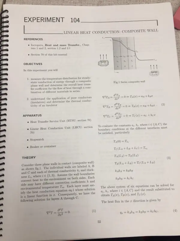
Transcribed Image Text:
EXPERIMENT 104.
LINEAR HEAT CONDUCTION: COMPOSITE WALL
REFERENCES
Incropera, Heat and mass Transfer., Chap-
ters 1 and 2, section 1.2 and 2.1
Section 70 of this lab manual
OBJECTIVES
In this experiment you will
1. measure the temperature distribution for steady-
state conduction of energy through a composite
plane wall and determine the overall heat trans-
fer coefficient for the flow of heat through a com-
bination of different materials in series.
2. understand the application of poor conductors
(insulators) and determine the thermal conduc-
tivity of an insulator
T
T
ム
A
4
A
c
111
Th
Fig. 1 Series composite wall
d²TA
dz2
VTA- -0 TA(a) a+b
V2To
dTa
= =0 Ta(z) ap+bg.
da
(2)
V2Tc
dB Te
dzB
-0 Tc(2) ac + box
APPARATUS
Heat Transfer Service Unit (HTSU: section 70)
Linear Heat Conduction Unit (LHCU: section
70)
Stopwatch.
Beaker or container
THEORY
Consider three plane walls in contact (composite wall)
as shown fig.1. The individual walls are labeled A, B
and C and each of thermal conductivity k, and thick-
ness L, where ie (1,3). Assume the wall boundaries
convect heat to the environment on both sides. Each
side may have different convection coefficients h and
environmental temperature T. Each layer must sat-
isfy the heat conduction equation eq.1 whose solution
is a linear function in 2. Consequently, we have the
following solution for layers A through C.
=
FT
V2T=
მკ-2
=0.
(1)
To evaluate the constants a, b,, where i E (A,C) the
boundary conditions at the different interfaces must
be satisfied. particularly
TA(0) T
Te(LA+LB+Lc)=T
TA(LA) =TB(LA)
TB(LA+LB) Tc(LA + LB)
kaba =kBbB
kaba-kebc
The above system of six equations can be solved for
a, b, where ie {A,C) and the result substituted to
obtain TA(z), TB(z), and Tc(z).
The heat flux in the z direction is given by
q=kabд=kBbB = kcbc.
(4)
55
rection (in this case, the r direction). Consequently, in
For A-D slab heat flow, heat can flow only in one di-
the absence of heat sinks/sources in a layer, the heat
flux must remain a constant as it passes through the
convective air layer on the left, through each slab and
finally through the convective air layer on the right.
To simplify the solution for a composite wall (with no
internal heat source), a simplified relation between the
overall heat flux through the composite wall and the
given temperature gradient from one side of the com-
posite wall to the other is found to be
Q=U (T.-T..).
where U is the overall heat transfer coefficient
1
U =
LB
Le
+
+
kp
kc
PROCEDURE
Part A: The Overall Heat Transfer Coefficient
(5)
1. Clamp the intermediate Stainless Steel section
(not instrumented) between the heated and
cooled section of the linear heat conduction unit
(LHCU) having lightly coated the mating faces:
with thermal paste. Connect the thermocouples
to the appropriate sockets on the front of the
service unit.
2. Start the computer. Start the heat transfer
service unit (HTSU) using the power switch
MAINS. Set the selector switch to "Automatic",
then start the ArmSoft software and select "Ex-
ercise C".
3. The Mimic Diagram is the most commonly used
display of the software, it gives a pictorial rep-
resentation of the equipment, with continuously
updated display boxes for all the various sensor
readings, calculated variables etc. To view the
Mimic Diagram, click Diagram from the View
drop down menu.
4. In order to establish communication between the
software and HTSU, click on the "Power On"
switch on the software diagram window
5. Open the water supply valve on the main sup-
ply hose, then adjust the flow control valve (not
the pressure regulator) to give approximately 1.5
litres/min. The actual flow can be checked using
a stopwatch and a measuring cylinder.
6. Use the heater control box on the mimic diagram
screen to adjust the percentage of full scale until
the voltage display box reads 9 volts
7. Allow the LHCU to stabilise (at least 15 mins).
Monitor the temperatures on the software mimic
diagram screen to determine when the tem-
peratures reach steady state (use "VIEW" and
"SHOW HISTORY" buttons, as well as "VIEW"
and "SHOW GAUGE" buttons).
8. When the temperatures have reached steady
state, select the icon "GO" to record one set
of data, which includes the following: Ti, Ta
Ta. To. T. Ts. V, I. Use button "VIEW" and
"PLOT RESULTS" to plot results and check if
the measured points form a straight line. You
can check results by looking at the "VIEW" and
"TABLE" buttons.
9. Set the heater to 12 volts using the same method
as before. Allow the LHCU to stabilise then re-
peat the above readings. Use buttons "SAM-
PLE" and "NEXT RESULTS" to enable the
"GO" button.
10. Save the results of measurements using the com-
mand "save as" from the file menu. Make sure
that you specify excel format (filename.xls).
11. After completion of all measurements turn off
the "Power On" button on the software screen,
power button MAINS on the HTSU and turn off
the water supply valve on the supply hose.
Notes:
The distance between each thermocouple is
0.015 m. The distance between thermocou-
ple Ts, or Te and the end face is 0.0075 m.
The thermal conductivity of the Brass sec-
tions is approximately 121 W/m°C, and
that of Stainless steel is approximately
25 W/m°C
For this experiment the following constants
are applicable:
Distance between thermocouples
Ty and the bot face
Distance between hot face
and cold face
Distance between the cold face
and thermocouple T
Thot 0.0375 m
int=0.030 m
cold 0.0375 m
Diameter of the bar
D=0.025 m
56
APPLICATION OF THEORY
Measurement errors: Temperature is measured
with accuracy of ±0.1°C. Voltage is measure with ac-
curacy of ±0.1V. Current is measured with accuracy
of ±0.1A. Linear dimensions are known with accuracy
of ±0.2mm. Position of thermocouples is known with
accuracy of +0.3mm.
Part A: The Overall Heat Transfer Coefficient
1. Estimate the cumulative influence of the exper-
imental errors on your calculated values for Q.
ATIs, khot, R and U.
2. Compare the two values obtained for the overall
heat transfer coefficient. Um and U, and comment
on any difference in the values obtained.
3. Plot a graph of temperature versus position
along the bar and draw the best straight line
through the points for the heated section and the
cooled section. Extrapolate each line to the joint
with the intermediate section then join these
these two points to give the gradient through
the intermediate section. Your results should
give values of approximately 25 W/m°C for the
thermal conductivity of Stainless Steel, assum-
ing no heat loss from the equipment. As a small
amount of heat loss is inevitable as the tempera-
ture of the bar increases, the calculated value for
the conductivity will increase at higher operating
temperatures.
4. What was the effect of varying the heater power
(heat flow through teh composite bar).
EXPERIMENT 104.
LINEAR HEAT CONDUCTION: COMPOSITE WALL-PRELAB
1. Read the Lab Manual write-up on this experiment along with the sections from your class textbook listed
in the references section. NOTE: This PRELAB is due at the beginning of the lab.
2. What is the objective of this experiment?
3. Solve the system of equations eq.2 for TA(a), Tn(x), and Te(2) given the boundary conditions eq.3.
4. Prove the result of eq.6.
59
NAME
DATE
GRADE
check_circle الجواب — حل مفصل خطوة بخطوة
hourglass_top
🔒
الحل الكامل متاح للمشتركين
اشترك في أرشيف الأسئلة لعرض هذا الحل وآلاف الحلول المفصلة خطوة بخطوة من معلمين معتمدين.