تم الحل ✓
categoryإحصاء
schoolبكالوريوس
event_available2026-07-13
السؤال
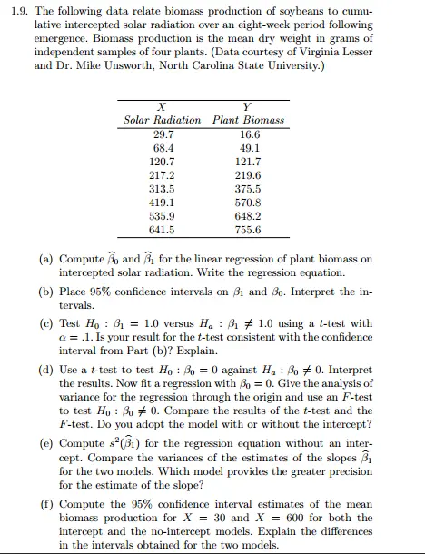
Transcribed Image Text:
1.9. The following data relate biomass production of soybeans to cumu-
lative intercepted solar radiation over an eight-week period following
emergence. Biomass production is the mean dry weight in grams of
independent samples of four plants. (Data courtesy of Virginia Lesser
and Dr. Mike Unsworth, North Carolina State University.)
X
Y
Solar Radiation Plant Biomass
29.7
16.6
68.4
49.1
120.7
121.7
217.2
219.6
313.5
375.5
419.1
570.8
535.9
648.2
641.5
755.6
(a) Compute B and B for the linear regression of plant biomass on
intercepted solar radiation. Write the regression equation.
(b) Place 95% confidence intervals on 31 and 30. Interpret the in-
tervals.
(c) Test Ho₁ = 1.0 versus Ha B₁ 1.0 using a t-test with
a = .1. Is your result for the t-test consistent with the confidence
interval from Part (b)? Explain.
(d) Use a t-test to test Ho: 30 = 0 against Ha: Bo 0. Interpret
the results. Now fit a regression with 30 = 0. Give the analysis of
variance for the regression through the origin and use an F-test
to test Ho Bo 0. Compare the results of the t-test and the
F-test. Do you adopt the model with or without the intercept?
(e) Compute s²(31) for the regression equation without an inter-
cept. Compare the variances of the estimates of the slopes
for the two models. Which model provides the greater precision
for the estimate of the slope?
(f) Compute the 95% confidence interval estimates of the mean
biomass production for X = 30 and X = 600 for both the
intercept and the no-intercept models. Explain the differences
in the intervals obtained for the two models.
1.12. Obtain the normal equations and the least squares estimates for the
model
Y₁ =+ẞixi + €i,
where x = (XX). Compare the results to equation 1.6. (The
model expressed in this form is referred to as the "centered" model;
the independent variable has been shifted to have mean zero.)
1.13. Recompute the regression equation and analysis of variance for the
Heagle ozone data (Table 1.1) using the centered model,
Y₁ = μ + B₁xi +εi,
where x = (XX). Compare the results with those in Tables 1.2
to 1.4.
1.14. Derive the normal equation for the no-intercept model, equation 1.40,
and the least squares estimate of the slope, equation 1.41.
1.15. Derive the variance of B₁ and Ŷ; for the no-intercept model.
1.16. Show that
(X-X)(-)=(X-X) = X(-Y).
1.19. The data in the table relate seed weight of soybeans, collected for
six successive weeks following the start of the reproductive stage, to
cumulative seasonal solar radiation for two levels of chronic ozone
exposure. Seed weight is mean seed weight (grams per plant) from
independent samples of four plants. (Data courtesy of Virginia Lesser
and Dr. Mike Unsworth.)
Low Ozone
Radiation Seed Weight
High Ozone
Radiation Seed Weight
118.4
.7
109.1
1.3
215.2
2.9
199.6
4.8
283.9
5.6
264.2
6.5
387.9
8.7
358.2
9.4
451.5
12.4
413.2
12.9
515.6
17.4
452.5
12.3
(a) Determine the linear regression of seed weight on radiation sep-
arately for each level of ozone. Determine the similarity of the
two regressions by comparing the confidence interval estimates
of the two intercepts and the two slopes and by visual inspection
of plots of the data and the regressions.
(b) Regardless of your conclusion in Part (a), assume that the two
regressions are the same and estimate the common regression
equation.
check_circle الجواب — حل مفصل خطوة بخطوة
hourglass_top
🔒
الحل الكامل متاح للمشتركين
اشترك في أرشيف الأسئلة لعرض هذا الحل وآلاف الحلول المفصلة خطوة بخطوة من معلمين معتمدين.