تم الحل ✓
categoryالرياضيات
schoolبكالوريوس
event_available2026-07-16
السؤال
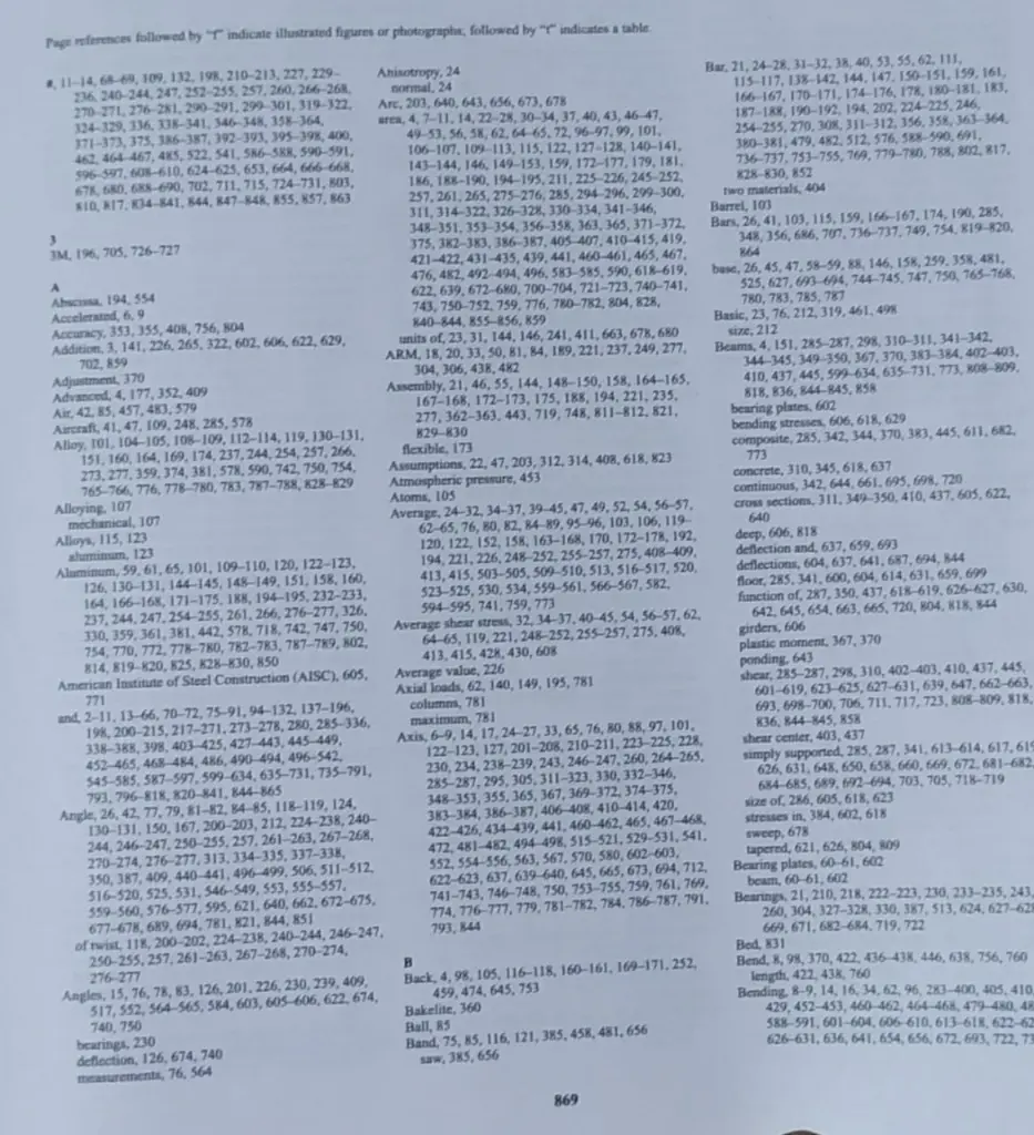
Transcribed Image Text:
3
Page references followed by "T" indicate illustrated figures or photographs, followed by "" indicates a table.
11-14, 68-69, 109, 132, 198, 210-213, 227, 229-
236, 240-244, 247, 252-255, 257, 260, 266-268,
270-271, 276-281, 290-291, 299-301, 319-322,
324-329, 336, 338-341, 346-348, 358-364,
371-373, 375, 386-387, 392-393, 395-398, 400,
462, 464-467, 485, 522, 541, 586-588, 590-591,
596-597, 608-610, 624-625, 653, 664, 666-668,
678, 680, 688-690, 702, 711, 715, 724-731, 803,
810, 817, 834-841, 844, 847-848, 855, 857, 863
3M, 196, 705, 726-727
A
Abscissa, 194, 554
Accelerated, 6, 9
Accuracy, 353, 355, 408, 756, 804
Addition, 3, 141, 226, 265, 322, 602, 606, 622, 629,
702, 859
Adjustment, 370
Advanced, 4, 177, 352, 409
Air, 42, 85, 457,483, 579
Aircraft, 41, 47, 109, 248, 285, 578
Alloy, 101, 104-105, 108-109, 112-114, 119, 130-131,
151, 160, 164, 169, 174, 237, 244, 254, 257, 266,
273,277, 359, 374, 381, 578, 590, 742, 750, 754,
765-766, 776, 778-780, 783, 787-788, 828-829
Alloying, 107
mechanical, 107
Alloys, 115, 123
aluminum, 123
Aluminum, 59, 61, 65, 101, 109-110, 120, 122-123,
126, 130-131, 144-145, 148-149, 151, 158, 160,
164, 166-168, 171-175, 188, 194-195, 232-233,
237, 244, 247, 254-255, 261, 266, 276-277, 326,
330, 359, 361, 381, 442, 578, 718, 742, 747, 750,
754, 770, 772, 778-780, 782-783, 787-789, 802,
814, 819-820, 825, 828-830, 850
American Institute of Steel Construction (AISC), 605,
771
and, 2-11, 13-66, 70-72, 75-91, 94-132, 137-196,
198, 200-215, 217-271, 273-278, 280, 285-336,
338-388, 398, 403-425, 427-443, 445-449,
452-465, 468-484, 486, 490-494, 496-542,
545-585, 587-597, 599-634, 635-731, 735-791,
793, 796-818, 820-841, 844-865
Angle, 26, 42, 77, 79, 81-82, 84-85, 118-119, 124,
130-131, 150, 167, 200-203, 212, 224-238, 240-
244, 246-247, 250-255, 257, 261-263, 267-268,
270-274, 276-277, 313, 334-335, 337-338,
350, 387, 409, 440-441, 496-499, 506, 511-512,
516-520, 525, 531, 546-549, 553, 555-557,
559-560, 576-577, 595, 621, 640, 662, 672-675,
677-678, 689, 694, 781, 821, 844, 851
of twist, 118, 200-202, 224-238, 240-244, 246-247,
250-255, 257, 261-263, 267-268, 270-274,
276-277
Angles, 15, 76, 78, 83, 126, 201, 226, 230, 239, 409,
517, 552, 564-565, 584, 603, 605-606, 622, 674,
740, 750
bearings, 230
deflection, 126, 674, 740
measurements, 76, 564
Anisotropy, 24
normal, 24
Arc, 203, 640, 643, 656, 673, 678
area, 4, 7-11, 14, 22-28, 30-34, 37, 40, 43, 46-47,
49-53, 56, 58, 62, 64-65, 72, 96-97, 99, 101,
106-107, 109-113, 115, 122, 127-128, 140-141,
143-144, 146, 149-153, 159, 172-177, 179, 181,
186, 188-190, 194-195, 211, 225-226, 245-252,
257, 261, 265, 275-276, 285, 294-296, 299-300,
311, 314-322, 326-328, 330-334, 341-346,
348-351, 353-354, 356-358, 363, 365, 371-372,
375, 382-383, 386-387, 405-407, 410-415, 419,
421-422, 431-435, 439, 441, 460-461, 465, 467,
476, 482, 492-494, 496, 583-585, 590, 618-619,
622, 639, 672-680, 700-704, 721-723,740-741,
743, 750-752, 759, 776, 780-782, 804, 828,
840-844, 855-856, 859
units of, 23, 31, 144, 146, 241, 411, 663, 678, 680
ARM, 18, 20, 33, 50, 81, 84, 189, 221, 237, 249, 277,
304, 306, 438, 482
Assembly, 21, 46, 55, 144, 148-150, 158, 164-165,
167-168, 172-173, 175, 188, 194, 221, 235,
277, 362-363, 443, 719, 748, 811-812, 821,
829-830
flexible, 173
Assumptions, 22, 47, 203, 312, 314, 408, 618, 823
Atmospheric pressure, 453
Atoms, 105
Average, 24-32, 34-37, 39-45, 47, 49, 52, 54, 56-57,
62-65, 76, 80, 82, 84-89, 95-96, 103, 106, 119-
120, 122, 152, 158, 163-168, 170, 172-178, 192,
194, 221, 226, 248-252, 255-257, 275, 408-409,
413, 415, 503-505, 509-510, 513, 516-517, 520,
523-525, 530, 534, 559-561, 566-567, 582,
594-595, 741, 759, 773
Average shear stress, 32, 34-37, 40-45, 54, 56-57, 62,
64-65, 119, 221, 248-252, 255-257, 275, 408,
413, 415, 428, 430, 608
Average value, 226
Axial loads, 62, 140, 149, 195, 781
columns, 781
maximum, 781
Axis, 6-9, 14, 17, 24-27, 33, 65, 76, 80, 88, 97, 101,
122-123, 127, 201-208, 210-211, 223-225, 228,
230, 234, 238-239, 243, 246-247, 260, 264-265,
285-287, 295, 305, 311-323, 330, 332-346,
348-353, 355, 365, 367, 369-372, 374-375,
383-384, 386-387, 406-408, 410-414, 420,
422-426, 434-439, 441, 460-462, 465, 467-468,
472, 481-482, 494-498, 515-521, 529-531, 541,
552, 554-556, 563, 567, 570, 580, 602-603,
622-623, 637, 639-640, 645, 665, 673, 694, 712,
741-743, 746-748, 750, 753-755, 759, 761, 769,
774, 776-777, 779, 781-782, 784, 786-787, 791,
793, 844
B
Back, 4, 98, 105, 116-118, 160-161, 169-171,252,
459, 474, 645, 753
Bakelite, 360
Ball, 85
Band, 75, 85, 116, 121, 385, 458, 481, 656
saw, 385, 656
Bar, 21, 24-28, 31-32, 38, 40, 53, 55, 62, 111,
115-117, 138-142, 144, 147, 150-151, 159, 161,
166-167, 170-171, 174-176, 178, 180-181, 183,
187-188, 190-192, 194, 202, 224-225,246,
254-255, 270, 308, 311-312, 356, 358, 363-364,
380-381, 479, 482, 512, 576, 588-590, 691,
736-737, 753-755, 769, 779-780, 788, 802, 817,
828-830, 852
two materials, 404
Barrel, 103
Bars, 26, 41, 103, 115, 159, 166-167, 174, 190, 285,
348, 356, 686, 707, 736-737, 749, 754, 819-820,
864
base, 26, 45, 47, 58-59, 88, 146, 158, 259, 358, 481,
525, 627, 693-694, 744-745, 747, 750, 765-768,
780, 783, 785, 787
Basic, 23, 76, 212, 319, 461, 498
size, 212
Beams, 4, 151, 285-287, 298, 310-311, 341-342,
344-345, 349-350, 367, 370, 383-384, 402-403,
410, 437, 445, 599-634, 635-731, 773, 808-809,
818, 836, 844-845, 858
bearing plates, 602
bending stresses, 606, 618, 629
composite, 285, 342, 344, 370, 383, 445, 611,682,
773
concrete, 310, 345, 618, 637
continuous, 342, 644, 661, 695, 698, 720
cross sections, 311, 349-350, 410, 437, 605, 622,
640
deep, 606, 818
deflection and, 637, 659, 693
deflections, 604, 637, 641, 687, 694, 844
floor, 285, 341, 600, 604, 614, 631, 659, 699
function of, 287, 350, 437, 618-619, 626-627,630,
642, 645, 654, 663, 665, 720, 804, 818, 844
girders, 606
plastic moment, 367, 370
ponding, 643
shear, 285-287, 298, 310, 402-403, 410, 437, 445,
601-619, 623-625, 627-631, 639, 647, 662-663,
693, 698-700, 706, 711, 717, 723, 808-809, 818,
836, 844-845, 858
shear center, 403, 437
simply supported, 285, 287, 341, 613-614, 617, 615
626, 631, 648, 650, 658, 660, 669, 672, 681-682
684-685, 689, 692-694, 703, 705, 718-719
size of, 286, 605, 618, 623
stresses in, 384, 602, 618
sweep, 678
tapered, 621, 626, 804, 809
Bearing plates, 60-61, 602
beam, 60-61, 602
Bearings, 21, 210, 218, 222-223, 230, 233-235, 243
260, 304, 327-328, 330, 387, 513, 624, 627-62
669, 671, 682-684, 719, 722
Bed, 831
Bend, 8, 98, 370, 422, 436-438, 446, 638, 756, 760
length, 422, 438, 760
Bending, 8-9, 14, 16, 34, 62, 96, 283-400, 405, 410
429, 452-453, 460-462, 464-468, 479-480, 48
588-591, 601-604, 606-610, 613-618, 622-62
626-631, 636, 641, 654, 656, 672, 693, 722, 73
869
SAL - NO
Mama L144SS
1-15-2426
21, 23, 244 132 379 M
47 24
- No 42 x
L
KARA 154, 226 2
RM42
37, 45-442 443 444
139-721 74, 750-75
Mus&277, 422-804
252 256 257 27 435, 454, 770
45, 101, 113, 114, 122, 170031
9, 101, 187 (25-425, 127, 879
M21 291, 404, M
Md 25, 2-4
M
2943017121 391 392 422 40, 4
74, 772-721-414 A
121 i 177, 200, 25, 41-442
79, 71, 771, 781 745-467
402, 04-3, 49, 853
796-400, 516-7, 8-4
367 360-372 24-NO-M
204 4%, 4R
4644044
44 445 44, 467 541, 600-44, 606,
349-353
A 31-325, 300 10-15
345, 36, 367, 332 JN 175 383 384 387
406-40 40-4144204-06 415 430
440 445 46 46 47, 541, 42-600,
LEK-64, 712, 142, 44,
Newton 39,212
helige M
Pa 134 446 41-422,153
320-32, 3, 42 44, 44
Pascal,
Pomgen 40
Pulal 526
2449
Period 121, 102, 125
homas, 102, 105, 12, 124
126-128, 110 19.200-271,271-813
p12-31
54-15 94,445, 72 81,
113-114131, 1,
41-46, 745-258
776-7785-79, 8M
Pipi 14.21.40, 41, 5, 1401 112 JA
44442M
748, 79, 121, X25
dations 114, 3, 2, 140, 175-174128
Pipes 189 194
Normal X 14 16 17,21-231, 38-459, 47.
4953-52, 54, 56-58 60 64-45, 75-89
95-96 118 117, 128, 125, 127, 130, 14
147 149 158, 143-168, 170, 172-178, 187,
343-325 317-318 321-322 113-1140
343-198865-366 30-371, 373-375-3
422, 456-415, 45-49 460 462 464-46 470
473-476, 480 482-48341-449-51 52-42, 4
523-527, 530, 534-533,540, 545-547, 353-555,
537-562 566-471, 584-586, 582-991, H2, 509,
614-419 420 421, 626-627, 714, 741, 79
804, 821
Plast m 545-547.356-554 256-561-6
34
Not al 316, 673
23, 142, 227, 672
640
Nylon 107
C
940,595
572-574 576 176, 182, 52, 588
621, 813
P, 21, 32, 34, 6284404
454 444 43015 M
5541 580-581,622
Plast 47
Plastic
defienation,
1, 1, 12, 504-500, 50
10477,772
677
Modeling 264, 763, 804
Mf 104-109 111-014, 118, 120, 123-128,
131, 141, 143, 146, 149, 152-153, 183, 165, 167,
173-175 190 225 226 264 268, 276, 342, 364
17-571, 576 57 579 44 64, 655, 657
684-685692, 71, 72, 740 741, 142, 772, WIZ
K00-42), 137, 544.855, 859
106-107, 109, 112-113, 128
day, 118, 123-124,640
11, 12, 124-125, 127, 131, 141, 143, 144
152-153, 163, 167, 173-175, 190, 225-226, 229
342, 376-471, 376-57,579, 594,640, 655,657
684-685, 92 700, 71, 723, 740-141, 72, 772
02 42-423,837, 844, 855, 859
Modula
106-107, 109 112-413, 128
nipdity, 118, 123-124
mptus, 254, 26, 308, 373
gh, 107, 109, 112-114, 128
ina 205-208, 210-211, 225, 228-229
317-323, 330, 334, 336, 138, 344, 146, 348,371,
407, 410-411,414,422, 424-426 433, 435,439,
Objectives)
Object 822 825
Observations, 201, 311-312, 569
Offer, 101, 107-108, 114, 121, 452
451-410.234.2 38. 46-48, 17, 61, 75,
77-7995-96, 106-102, 105, 121, 123, ET, LM
140-143, 152, 155, 157, 160-165, 174, 171, 184,
188-189, 192, 194 217, 223-226, 238, 240, 245
24, 251, 254 256, 261 268, 270-271 285-297
295-296 298, 31, 328, 333-335, 137, HC-144
346, 358 408, 422 434, 460-461, 494-495, 529
54, 554, 562, 570 582-585 590, 47, 613-614
695,647 698, 707, 130-721, 744-145, 75-752
754-755, 759, 765-766 769-771, 802-85, 809,
815-836,853
Open 436, 438, 446 457, 463, 481, K21
Optical
Optimum, 459
Onder 4-7, 9, 15, 47, 59, 62, 76, 78-79, 89, 10,
116, 122, 155-156, 166, 17, 182, 185, 226
234-239, 24, 266, 272, 286-287 291-292348
322.343-345 391, 353, 371, 418 422, 431, 431,
453, 466, 547, 605-606, 618 622-623, 631, 641.
647, 661, 663, 64, 701, 71, 710, 734, 770, 773
833, 647-848 854
Ordiner, 194, 554
Play 126
Post 4-1,9-8, 12, 15-222-
0-4-SCHRAM
10-119, 112 116-119 126-128, 138, 14-12
145, 13, 14, 16 17 18 182, 134 1
190-196 398 214-218-216 28 28 288
246-34, 25, 261, 20-34, 290, 20-28
297-29 1 113-315317-334 1332-134
127, 334-375, 308 340-30 MM
383-355, 258 36C 364 371-17 J
407-410 414-418 437-42 443 444 4
43-467 49-471, 413-475 477-40 40
491-445, 500-301, 57-823, 525
539-542-345-546 950-362, 961-337D-STA
563, 585-5510-5, 64, 60-61 462
672-478 685 -4 0 2 18 TO
720-721, 7, 78, 70, 415-412, 6, 416-415
841-842 346-4118-AT MY
Pom 3-4817-182
83, 97, 107, 125-131, 12, 288-
199, 17, 181, 208 230-211,211-852 24
218 245-24 20, 252 297 298 26-387
318, 326-321, 134, 136-127 318 34 36 38
362-363 370 382, 18409-41944
434-415, 48, 40-441 462 473-47, 48,
873
444
WA
RANCHO
LONAS
from cent
vertical c
slopes of
horizonta
(Section
slope). T
1:1.5. For
45°); for
Wh
For exar
Side slo
represen
the slope
Aft
determi
lated ve
Fo
are de
section
param
profile
FIGURE 16.34 (c) Perspective view of a DTM projected on a video screen. (Courtesy
of Integraph Corporation.)
superi
necess
stakes
comp
for su
002
A horizontal or geodetic datum consists of an ellipsoid of revolution approximating the
figure of the earth and a set of constants or constraints that specify the size, position, and
orientation of the ellipsoid. Two of the constants define the semimajor axis and the
flattening of the ellipsoid. The position is often given indirectly by three constants E., Ma
and N. at an origin point, O, where &, represents the deflection of the vertical in the meridian
plane, n, represents the the deflection of the vertical in the prime vertical plane, and N
represents the difference between the geoid and the ellipsoid, which is also called the geoid
undulation. In addition to these three constants, an observed astronomic latitude and either
an observed astronomic longitude or an astronomic azimuth would define the geodetic
latitude and longitude of the origin point. More recent datums define the ellipsoid position
by specifying that it coincide with the center of mass of the earth. An example of the earlier
type of horizontal datum is the North American datum of 1927 (NAD 27), which was based
on an origin point at Meades Ranch, Kansas, and used the Clarke 1866 ellipsoid with
a = 6,378,206.4 meters and b = 6,356,583.8. This was the basis for most mapping done
in the United States until recently. A general readjustment including satellite observations
and very long base-line interferometry has resulted in the North American datum of 1983
(NAD 83), which is an example of the latter type of geodetic or horizontal datum. It is based
on the geodetic reference system of 1980 (GRS 80) ellipsoid with a = 6,378,137.0 and
1/f = 1/298.257522101. The adoption of GRS 80 for the NAD 83 is a favorable circum-
stance for users of the GPS system. The world geodetic system of 1984 (WGS 84), as used
in GPS computations, essentially is the same as GRS 80.
A vertical datum is the surface to which elevations or depths are referred. Prior to 1991,
all surveys and mapping in the conterminous United States were based on the national
geodetic vertical datum of 1929, formerly called the sea-level datum of 1929. This datum
was based on a least-squares adjustment to 26 mean sea-level tide stations (Zilkosky,
Richards, and Young, 1992) in the United States and Canada and was the result of a general
adjustment of level networks in the United States and Canada in 1929. In 1991, the National
Geodetic Survey completed incorporating new data into the existing survey network, result-
ing in the North American vertical datum of 1988 (NAVD 88). Elevations used in topo-
graphic mapping, geodetic surveys, engineering studies, engineering construction surveys,
and geographic information systems should be referred to the current national vertical
datum, NAVD 88. The NAVD 88 is not a mean sea-level datum and should not be confused
with local mean sea-level datums. The national datum was determined by a minimal
constraint adjustment, holding fixed the height of a primary tidal bench mark at Father Point
(Pointe au Pere), Rimouski, Quebec, Canada. Canadian-Mexican-U.S. leveling observa-
tions were included in this adjustment. Consequently, small differences exist between the
national datum and local mean sea-level for a specific location.
and A
Elevations used in boundary surveys are often referred to a tidal datum in tidal waters
or the lake level in the Great Lakes regions. Tidal datums are defined by the phase of the
tide, described as mean high water, mean low water, and mean lower low water. Caution
always should be exercised to ensure that bench marks and control points refer to the same
datum, particularly in areas where multiple datums are known to exist.
Other horizontal and vertical datums are employed for Alaska (vertical datum), Puerto
Rico, the Virgin Islands, Guam, and other oceanic islands. Specifications for these datums
can be obtained by requesting information from the National Geodetic Survey.
(X, Y) or eastings and northings (E, N). This is necessary both for preparing hard-copy
maps and for representing map data digitally in a geographic information system. Eventu
ally GIS systems may accommodate latitude and longitude, but at present they generally
require Cartesian coordinates. As described in Chapter 11, map projections include the
Lambert conformal conic and the transverse Mercator. The newer U.S.G.S. quadrangle
maps are on the universal transverse Mercator (UTM) projection (Section 11.14). Older
quadrangle maps employed the polyconic projection (Section 11.9). The state plane coor-
dinate systems (SPCS), based on the Lambert conformal conic or the transverse Mercator
projections, are widely used as reference coordinates for mapping and GIS. For regional or
statewide projects that may cover multiple state plane zones, the UTM projection often is
used. For special circumstances, a unique projection can be defined for a particular project,
although data interchange is facilitated by using standard projections wherever possible.
14.4
TOPOGRAPHIC MAPS
A topographic map shows, through the use of suitable symbols, (1) the spatial characteris-
tics of the earth's surface, with such natural features as hills and valleys, vegetation and
rivers; and (2) constructed features such as buildings, roads, canals, and cultivation. The
distinguishing characteristics of a topographic map, as compared with other maps, is the
representation of the terrain relief.
Topographic maps are used in a variety of ways. They are necessary in the design of
any engineering project that requires the consideration of elevations for gradients. They
also are used for delineating the extent of a flood plain, planning for economic development,
and managing natural resources.
The preparation of general topographic maps traditionally has been a function of
governmental agencies. However, the rapid development of computer-based tools for ter-
rain modeling and the increasing availability of high-quality field data enable nearly any
user of topographic information to create detailed, specialized topographic maps using a
desktop computer.
The principal source of topographic data in the United States remains the national map
series of medium (1:24,000) to small (1:1 million) scale topographic maps prepared by the
National Mapping Division of the U.S. Geological Survey (Figure 14.1). These maps cover
the entire United States and its territories in quadrangle tiles from 7' x 7' in latitude
and longitude at a map scale of 1:24,000 to tiles 4° x 12° in extent at a scale of 1:1 million.
These topographic maps have been compiled using field survey data and photogrammetric
compilation techniques. Recently, the U.S.G.S. also provided the same data contained in
the printed map series in digital form as digital line graph (DLG) files. Although the printed
maps are regularly photo revised, it is common for the latest quadrangle maps not to have
been revised in several years. For engineering applications in rapidly developing areas, this
time lag may not be acceptable.
The U.S.G.S. currently is in the process of developing a new, large-scale digital
orthophoto quadrangle (DOQ) and quarter-quad (DOQQ) map series for the entire coun-
try. These new orthophoto maps will be generated at scales of 1:24,000 and 1:12,000,
respectively. The DOQQ maps will have a 1-m ground sample (pixel) resolution and will
be provided in a UTM system based on NAD 83. The status of the DOQ mapping program
is shown graphically in Figure 14.2. The new map series combines the information content
of a photograph and the geometric qualities of a standard map and will be uniquely suited
for use in spatial information systems. More information on these products is available from
the Earth Sciences Information Centers of the U.S.G.S. or by calling 1-800-USA-MAPS.
78
CH
Ma
M
Sp
Int
Sy
-3 m. Then
two edges. In Figure 14.6b, the contours cross a paved road with curbs. Most curbs are
0.15 m high, so the contour crosses the curb at right angles and runs along the face of the
curb until it reaches the contour elevation in the gutter line. Therefore, if the grade (Sec.
tion 3.8) of the road is 5 percent, the distance from where the contour crosses the top of the
curb to the point where it meets the contour elevation in the gutter is 0.15/0.05
the contour crosses the pavement slightly convex down the slope to the gutter line on the
other side, follows the face of the curb until the elevation at the top of the curb is reached,
and crosses the curb and sidewalk at right angles (assuming that the sidewalk is horizontal),
The contour interval in Figure 14.6a is 5 ft and that in Figure 14.6b is 2 m.
14.7
CHOICE OF MAP SCALE AND CONTOUR INTERVAL
Formerly, when a hard-copy map was the archival data record used to present the results
of a topographic survey, the choice of map scale and contour interval indeed was critical.
Current engineering practice often dictates that map data be recorded digitally, usually in
ground coordinate units. Thus, within limits, the hard-copy representation of the map can
be plotted at any scale desired. This capability is well known to users of CAD systems and
other computer graphics programs. Of course, such things as text annotation size and
placement, point and line symbology, and feature generalization are scale specific and do
not change with plot scale. So, for a map plotted at much smaller scale than intended, the
text would be unreadable. A portion of the same map plotted at much larger scale than
intended would be graphically unpleasing with the text too large. Likewise, the choice of
contour interval was once a fixed parameter of the data collection process. Currently, the
parameter that limits the fidelity of the representation of the ground surface often is the
density of points in the digital terrain model (DTM, see Section 14.8). This might include
the spacing of the points of known elevation or elevation "posts" in a grid layout, the density
of points of known spatial position or mass points for construction of a triangular irregular
network (TIN) (See Section 14.8), and the density and completeness of breaklines (Sec-
tion 14.9) and other subordinate features. Having selected the sampling criteria of the
terrain surface, a contour representation, again within limits, can be interpolated and plotted
at any desired interval. Computer mapping programs, quite readily, and inappropriately.
will produce 1-dm contours from data points 30-m apart and accurate to only 1 m.
Therefore, sound judgment should be used in selecting the sampling density of the terrain
points and a contour interval for interpolation and plotting. Hard-copy contour maps will
continue to be used for the foreseeable future, and it therefore is useful to look at some of
the design parameters used in their construction, in particular scale and contour interval.
Accuracy standards for engineering maps, presented later in this chapter (Sec-
tion 14.26), generally dictate that well-defined, plotted features should be located within
0.5 mm of their true position at the plotted map scale. Therefore, if a user needs point
positions accurate to 2.5 m, a map scale of 1:5000 is indicated. With regard to elevations,
accuracy standards generally require that interpolated heights be accurate to one-half
contour interval. Therefore, if one needs 0.25-m elevation accuracy, the contour interval
should be no greater than 0.5 m. Along with a given map scale, an implied level of detail
is expected by the user. Other factors that influence the choice of map scale are (1) the
clarity with which features can be shown. (2) the cost (the larger the scale, the higher is
the cost). (3) the consistency of the map with other adjoining or overlapping maps, (4) the
number and character of the features to be plotted, the nature of the terrain, and the contour
interval. Typical map scales, map uses, and corresponding contour intervals are shown in
Table 14.1.
A horizontal or geodetic datum consists of an ellipsoid of revolution approximating the
figure of the earth and a set of constants or constraints that specify the size, position, and
orientation of the ellipsoid. Two of the constants define the semimajor axis and the
flattening of the ellipsoid. The position is often given indirectly by three constants E., Mo
and N. at an origin point, O, where &, represents the deflection of the vertical in the meridian
plane, n, represents the the deflection of the vertical in the prime vertical plane, and N
represents the difference between the geoid and the ellipsoid, which is also called the geoid
undulation. In addition to these three constants, an observed astronomic latitude and either
an observed astronomic longitude or an astronomic azimuth would define the geodetic
latitude and longitude of the origin point. More recent datums define the ellipsoid position
by specifying that it coincide with the center of mass of the earth. An example of the earlier
type of horizontal datum is the North American datum of 1927 (NAD 27), which was based
on an origin point at Meades Ranch, Kansas, and used the Clarke 1866 ellipsoid with
a = 6,378,206.4 meters and b = 6,356,583.8. This was the basis for most mapping done
in the United States until recently. A general readjustment including satellite observations
and very long base-line interferometry has resulted in the North American datum of 1983
(NAD 83), which is an example of the latter type of geodetic or horizontal datum. It is based
on the geodetic reference system of 1980 (GRS 80) ellipsoid with a = 6,378,137.0 and
V/f = 1/298.257522101. The adoption of GRS 80 for the NAD 83 is a favorable circum-
stance for users of the GPS system. The world geodetic system of 1984 (WGS 84), as used
in GPS computations, essentially is the same as GRS 80.
A vertical datum is the surface to which elevations or depths are referred. Prior to 1991,
all surveys and mapping in the conterminous United States were based on the national
geodetic vertical datum of 1929, formerly called the sea-level datum of 1929. This datum
was based on a least-squares adjustment to 26 mean sea-level tide stations (Zilkosky,
Richards, and Young, 1992) in the United States and Canada and was the result of a general
adjustment of level networks in the United States and Canada in 1929. In 1991, the National
Geodetic Survey completed incorporating new data into the existing survey network, result-
ing in the North American vertical datum of 1988 (NAVD 88). Elevations used in topo-
graphic mapping, geodetic surveys, engineering studies, engineering construction surveys,
and geographic information systems should be referred to the current national vertical
datum, NAVD 88. The NAVD 88 is not a mean sea-level datum and should not be confused
with local mean sea-level datums. The national datum was determined by a minimal
constraint adjustment, holding fixed the height of a primary tidal bench mark at Father Point
(Pointe au Pere), Rimouski, Quebec, Canada. Canadian-Mexican-U.S. leveling observa-
tions were included in this adjustment. Consequently, small differences exist between the
national datum and local mean sea-level for a specific location.
and A
Elevations used in boundary surveys are often referred to a tidal datum in tidal waters
or the lake level in the Great Lakes regions. Tidal datums are defined by the phase of the
tide, described as mean high water, mean low water, and mean lower low water. Caution
always Radius of a curve is 230 m. What is the degree of the curve.
datum, particularly in areas where multiple datums are known to exist.
Other horizontal and vertical datums are employed for Alaska (vertical datum), Puerto
Rico, the Virgin Islands, Guam, and other oceanic islands. Specifications for these datums
can be obtained by requesting information from the National Geodetic Survey.
по
derivative of the terrain surface is not continuous; for example, along a ridge line or a drain
line. These data are not tied to a particular graphic representation. Implicitly associated
with the terrain data in a DTM is the interpolation algorithm used to reconstruct the terrain
surface. Second, the archival record is the digital coordinate file itself rather than a par-
ticular graphic depiction. Such graphical depictions as contours, profiles, or wire frame
perspective views can be generated as needed, but only the original terrain points and
features are considered to be archival data.
DTMs generally are organized such that the "mass points" lie in a regular grid pattern
or they represent vertices of local triangular patches in an array referred to as a triangulated
irregular network. Companies and government agencies seem to have developed institu-
tional preferences for one method or the other. Just as there are engineering design criteria
for selecting a contour interval to represent terrain for a given application, so too similar
criteria are used to select a point spacing so that the DTM adequately represents the terrain.
These criteria depend on the potential uses for the data, accuracy requirements, the terrain
character, and other factors. The advantages of a regular grid layout are a simplified data
collection routine, and ease of data access by subsequent programs. The disadvantages are
related mostly to the necessity to select a single grid interval, sufficient to define the terrain
in the roughest areas although likely to be oversampled in regions where the terrain is
smooth and featureless. Conversely, the merits of the irregular point approach are the mirror
image of those for the regular grid. The sampling interval can change to match the local
terrain character, introducing a kind of stratified sampling, optimizing the quantity of data
necessary to define the terrain. Data access for subsequent software analysis is considerably
more involved than when using the simple grid structure.
Ideally, during the design of a DTM database, a quantitative analysis is done to deter-
mine the magnitude of the errors expected during reconstruction of the terrain surface. The
magnitude of these errors should be within the error budget of potential user or client
applications. Interpolation methods for generating intermediate points can include patch-
wise polynomials, b-splines, moving surface methods, linear prediction with trend surfaces
and covariance functions (sometimes called summation of surfaces), bilinear methods,
plane triangle methods, and ideal reconstruction functions from signal theory. Given a
DTM database and an interpolation function, one should be able to construct a profile or
cross section along any arbitrary path within the area covered by the DTM. Likewise, one
should be able to interpolate heights at arbitrary points within the area covered. This
capability would permit one to interpolate heights at regular grid points from an irregular
grid as well as interpolate irregular points from a regular grid. Thus, with possibly some cost
to accuracy, one could convert between these two popular storage conventions. Converting
from irregular points to regular points is straightforward. Converting from regular gridded
points to irregular points often is more difficult, especially when there is a desire to reduce
drastically the number of points.
Another issue to consider when constructing or using DTM databases is the matter of
consistency between the terrain, as defined by the DTM, and the feature data, such as roads,
streams, and buildings. On a hard-copy map, these two classes of data always are implicitly
consistent. However, if they are collected and stored independently as 3D or 2.5D, then they
may be inconsistent or conflicting. This could occur if, for example, a road were above the
terrain surface or if a stream were placed so as apparently to flow uphill.
14.9
BREAKLINES AND OTHER TERRAIN FEATURES
Terrain data points, whether in a grid pattern or an arbitrary pattern, always will fail to
represent terrain fully in areas where there are sharp breaks or, more properly, discontinu-
ities in slope. Such discontinuities occur along ridge lines, at the upper and lower edges of
79
CH
M
M
Sp
In
Sy
TABLE 14.1
Typical map scales
Map scale
Typical uses
Contour interval for
nonmountainous terrain
1:1,000
Design
1:2,000
Design
1:5,000
Planning
0.25 m
0.5 m
Im
1:10,000
Planning
2 m
1:25,000
Regional planning
2.5 m
1:50,000
Regional planning
5 m
1:100,000
Regional planning
5 or 10 m
1:250,000
Regional planning
10 m
1:500,000
1:500,000
State planning
20 m
National planning
20 or 50 m
with
The choice of a proper contour interval for a topographic survey and map is based on
our principal considerations: (1) the desired accuracy of elevations to be determined from
he map, (2) the characteristic features of the terrain, (3) the legibility of the map, and
4) the cost. Assuming that heights can be interpolated to one-half of the contour interval,
then a map with a 1-m contour interval should yield more accurate heights than a map
a 2-m contour interval. Terrain areas with a fine-textured surface may require a smaller
contour interval to represent it than otherwise would be necessary. Contours should not be
so close together as to obscure other important map features, although cartographic design
and selection of colors, saturations, and line weights can significantly influence the map
legibility. Smaller contour intervals, in general, cost more assuming that the conventional
accuracy levels are maintained.
As shown in Table 14.1, smaller map scales generally are associated with larger
contour intervals. Traditionally, maps have been classified according to scale as large,
medium, and small, with these categories generally as in Table 14.2.
The American Society of Civil Engineers' (ASCE) Surveying and Mapping Division
has a more detailed classification for map scales and contour intervals.
1. Design maps. These maps are used in the design and construction of specific engineering
work of all kinds. Scales vary from 1:100 to 1:2000, with contour intervals from 0.1 to
1 m, depending on the type of project, land use, and terrain characteristics. Two subcat-
egories are given within this group. Critical design maps are used on projects having
critical space, orientation, position, or elevation restrictions; for example, a highway
interchange in an urban area. General design maps are prepared for projects that have
no such rigid restrictions with respect to location; for example, a map prepared for a rural
water distribution system.
2. Planning maps. These maps include a large group of maps used in planning engineering
work or in overall planning at the urban, regional, national, and international levels.
These maps may be used as a foundation for GIS, geological studies, land use, agricul-
tural production, population studies, public service planning, and atlases. These maps
generally fall in the medium- to small-scale range.
TABLE 14.2
Map-scale categories
Large scale
Medium scale
Small scale
1:20,000 and larger
1:20,000-1:50,000
1:50,000 and smaller
784
Greek
50
Slatt
20
ALTA
HILL
YER
The Oaks
Glenbrook
23
Hills Flat
Cardon
GRASSANES
South
13107
Union
Hill
35
STATE ISTORIC Puk
Cedar
Ridge
972
1213700
Nevada
City
FIGURE 14.1
Typical topographic map of the U.S. Geological Survey. Scale is 1:24,000 (2000 ft/in.). Contour Interval 20 ft. (U.S. Geological Survey.)
Peardale
43
GQ
(X, Y) or eastings and northings (E, N). This is necessary both for preparing hard-copy
maps and for representing map data digitally in a geographic information system. Eventu
ally GIS systems may accommodate latitude and longitude, but at present they generally
require Cartesian coordinates. As described in Chapter 11, map projections include the
Lambert conformal conic and the transverse Mercator. The newer U.S.G.S. quadrangle
maps are on the universal transverse Mercator (UTM) projection (Section 11.14). Older
quadrangle maps employed the polyconic projection (Section 11.9). The state plane coor-
dinate systems (SPCS), based on the Lambert conformal conic or the transverse Mercator
projections, are widely used as reference coordinates for mapping and GIS. For regional or
statewide projects that may cover multiple state plane zones, the UTM projection often is
used. For special circumstances, a unique projection can be defined for a particular project,
although data interchange is facilitated by using standard projections wherever possible.
14.4
TOPOGRAPHIC MAPS
A topographic map shows, through the use of suitable symbols, (1) the spatial characteris-
tics of the earth's surface, with such natural features as hills and valleys, vegetation and
rivers; and (2) constructed features such as buildings, roads, canals, and cultivation. The
distinguishing characteristics of a topographic map, as compared with other maps, is the
representation of the terrain relief.
Topographic maps are used in a variety of ways. They are necessary in the design of
any engineering project that requires the consideration of elevations for gradients. They
also are used for delineating the extent of a flood plain, planning for economic development,
and managing natural resources.
The preparation of general topographic maps traditionally has been a function of
governmental agencies. However, the rapid development of computer-based tools for ter-
rain modeling and the increasing availability of high-quality field data enable nearly any
user of topographic information to create detailed, specialized topographic maps using a
desktop computer.
The principal source of topographic data in the United States remains the national map
series of medium (1:24,000) to small (1:1 million) scale topographic maps prepared by the
National Mapping Division of the U.S. Geological Survey (Figure 14.1). These maps cover
the entire United States and its territories in quadrangle tiles from 7' x 7' in latitude
and longitude at a map scale of 1:24,000 to tiles 4° x 12° in extent at a scale of 1:1 million.
These topographic maps have been compiled using field survey data and photogrammetric
compilation techniques. Recently, the U.S.G.S. also provided the same data contained in
the printed map series in digital form as digital line graph (DLG) files. Although the printed
maps are regularly photo revised, it is common for the latest quadrangle maps not to have
been revised in several years. For engineering applications in rapidly developing areas, this
time lag may not be acceptable.
The U.S.G.S. currently is in the process of developing a new, large-scale digital
orthophoto quadrangle (DOQ) and quarter-quad (DOQQ) map series for the entire coun-
try. These new orthophoto maps will be generated at scales of 1:24,000 and 1:12,000,
respectively. The DOQQ maps will have a 1-m ground sample (pixel) resolution and will
be provided in a UTM system based on NAD 83. The status of the DOQ mapping program
is shown graphically in Figure 14.2. The new map series combines the information content
of a photograph and the geometric qualities of a standard map and will be uniquely suited
for use in spatial information systems. More information on these products is available from
the Earth Sciences Information Centers of the U.S.G.S. or by calling 1-800-USA-MAPS.
78
CH
Ma
M
Sp
Int
Sy
check_circle الجواب — حل مفصل خطوة بخطوة
hourglass_top
🔒
الحل الكامل متاح للمشتركين
اشترك في أرشيف الأسئلة لعرض هذا الحل وآلاف الحلول المفصلة خطوة بخطوة من معلمين معتمدين.