تم الحل ✓
categoryهندسة كهربائية
schoolبكالوريوس
event_available2026-07-15
السؤال
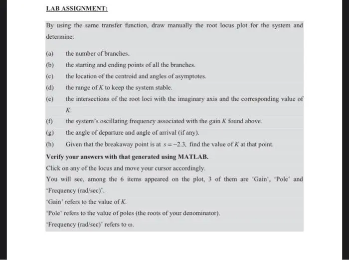
Transcribed Image Text:
LAB ASSIGNMENT:
By using the same transfer function, draw manually the root locus plot for the system and
determine:
the location of the centroid and angles of asymptotes.
(a)
the number of branches.
(b)
the starting and ending points of all the branches.
(c)
(d)
the range of K to keep the system stable.
(e)
(f)
the intersections of the root loci with the imaginary axis and the corresponding value of
K.
(h)
the system's oscillating frequency associated with the gain K found above.
Given that the breakaway point is at x=-2.3, find the value of K at that point.
the angle of departure and angle of arrival (if any).
Verify your answers with that generated using MATLAB.
Click on any of the locus and move your cursor accordingly.
You will see, among the 6 items appeared on the plot, 3 of them are 'Gain', 'Pole' and
*Frequency (rad/sec)*.
"Gain' refers to the value of K.
Pole' refers to the value of poles (the roots of your denominator).
"Frequency (rad/sec)' refers to to.
29
Lab Experiment: Introduction to Root Locus
Since the root locus is actually the locations of all possible closed loop poles, from the root locus
we can select a gain such that our closed-loop system will perform the way we want. If any of
the selected poles are on the right half plane, the closed-loop system will be unstable. The poles
that are closest to the imaginary axis have the greatest influence on the closed-loop response, so
even though the system has three or four poles, it may still act like a second or even first order
system depending on the location(s) of the dominant pole(s).
PLOTTING THE ROOT LOCUS OF A TRANSFER FUNCTION
Consider an open loop sem which has a transfer function of
KH(s)=-
K
s(s+3)(s²+2s+2)
How do we design a feed-back controller for the system by using the root locus ethod? Make a
MATLAB file called rl.m. Enter the transfer function and the command to the root locus:
% Create the numerator polynomial.
num = 1;
% Create the denominator polynomial, using the conv function. Conv takes vectors and
expands them.
den conv(conv([10],[13]),[122]);
% Create a new figure window to plot on. It will not overlap with the previous figure.
%provided that it is not labeled with the same number (i.e. figure(1), figure(2) etc).
figure(1)
% Plot the root locus with the command rlocus.
rlocus(num,den)
check_circle الجواب — حل مفصل خطوة بخطوة
hourglass_top
🔒
الحل الكامل متاح للمشتركين
اشترك في أرشيف الأسئلة لعرض هذا الحل وآلاف الحلول المفصلة خطوة بخطوة من معلمين معتمدين.