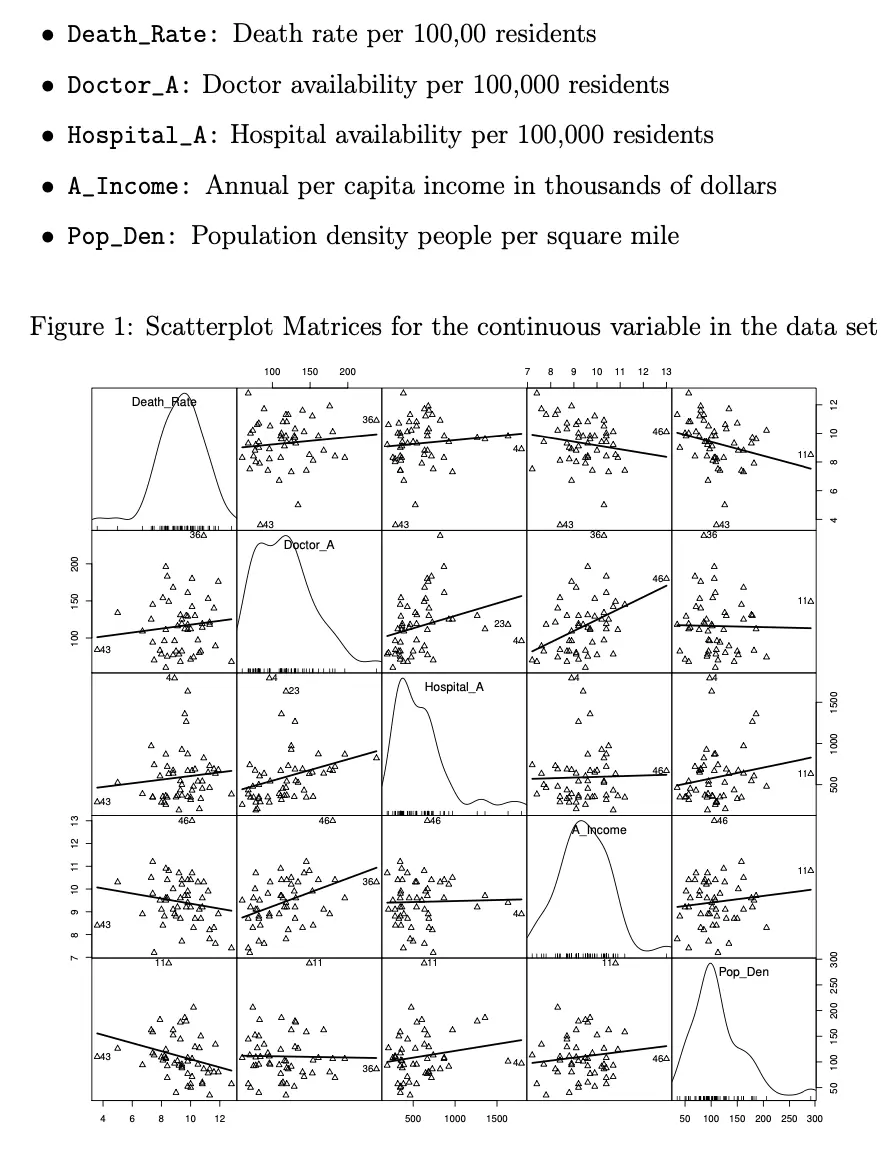
► • Death_Rate: Death rate per 100,00 residents • Doctor_A: Doctor availability per 100,000 residents • Hospital_A: Hospital availability per 100,000 residents • A_Income: Annual per capita income in thousands of dollars Pop Den: Population density people per square mile Figure 1: Scatterplot Matrices for the continuous variable in the data set 100 150 200 Δ Death Rate A 36A Δ Δ A Δ Δ ΔΔ Δ ΔΔ Δ Δ Δ Δ A43 36A 100 150 200 Δ Δ Δ Δ 100 ΔΔΔ Δ A43 A Δ 4A 3 - 443 N Δ Δ A4 Doctor_A 7 8 9 10 11 12 13 Δ Δ Δ Δ Δ 46444 Δ ΑΔ ΔΑ Δ Δ Δ A43 143 Δ 36A Δ A43 A36 11A Δ Δ Δ 46A Δ Δ 4 A A Δ Δ 114 ΔΙΔΑΝ 23A ΔΔ A A AA ΑΔ Δ A Δ AA Δ Hospital_A Δ Δ AA Δ A23 Δ Δ Δ Δ Δ D Δ A Δ 46A A46 46A D = AA Δ 10 9 A 443 00 Δ Δ ΔΑ A Δ Δ 4 Δ 36A ΔΕ Δ Δ ΔΔ Δ ΔΑ 4 ΔΔ 4 4 4 Δ ΑΔ Δ ΑΔ Δ Δ ΔΙ Δ11 Δ Δ Δ D Δ Δ Δ 44 Δ AA Δ 44 ΔΔ Δ ΔΑ A A 443 Δ 3644 Δ Δ T 4 6 8 10 12 Δ Δ 4A ΔΑ Δ 46A A Δ AA Δ AIncome 11A Δ ΔΑ Δ 44 Δ Δ Δ ΔΔ Δ ΔΑΔ Δ A 500 1000 1500 46A 50 ΔΑ A Δ A Δ Δ 446 Δ Δ Pop_Den Δ 11A 114 100 150 200 250 300 50 100 150 200 250 300 1000 1500 2 4 6 8 10 4. Using the data-set described in question 3. The following model is considered: = Death Rate, ẞo + B₁Doctor_A, + B₂Hospital_A; + B3A_Income, + B₁Pop_Den, + εi (2) for i=1,..., 53, where ; represents the error in the model. The estimated coeffi- cients and their standard errors are: coef Estimate Std. Error Во 12.26 2.02 ẞ1 0.007 0.006 B2 0.0005 0.0007 ẞ3 -0.33 0.23 B4 -0.009 0.004 (a) Interpret the estimated coefficients? [6] (b) Test and interpret the hypothesis Hoẞ3 = 0 against Ha: B3 # 0 using a t-test. Given that to.025,48 = 2.01. [4] (c) Test and interpret the following hypotheses, Ho: B3 = 34 = 0 using an F-test. Given that F0.05,2,48 3.19 and the ANOVA table below: Df Sum Sq Doctor_A 1 1.926 Hospital_A 1 0.918 A_Income 1 8.195 Pop_Den 1 9.614 Residuals 48 123.074 [6] (d) How would I modify the model in (2) to include the categorical variable State. The possible States in this data set are: Ohio, Indiana, Illinois, Iowa, Missouri, Nebraska, Kansas, and Oklahoma. [2] (e) Calculate and interpret the adjusted coefficient of multiple determination R²? [2] (f) Provide an interpretation of each of the diagnostic plots in Figure (2) for the regression model in (2) (i.e. provide a short description of what the plot can be used to assess and an interpretation for the particular plots provided). VIStandardized residualsl 0.0 0.5 1.0 1.5 Residuals T Q 2 7 0 Z- Figure 2: Diagnostic plots for the regression model in (2) Residuals vs Fitted 031 043 510 7.5 8.0 8.5 9.0 9.5 10.0 10.5 Fitted values ° Scale-Location 043 8 ° 031 510 Standardized residuals Standardized residuals 2 2 043 043 031 оо 00000 -2 -1 Normal Q-Q 0 Theoretical Quantiles Residuals vs Leverage 051 40 Cook's distance 7.5 8.0 8.5 9.0 9.5 10.0 10.5 0.00 0.05 0.10 0.15 0.20 0.25 0.30 0.35 Fitted values Leverage 2 0.5 0.5 510